• Programming Tool
• A-Z
• Pages
• Simulator
• Diagrams
• Scripts
• 

DIAGRAM display function

Contents of this document

1. Diagrams
   1. Introduction
2. Diagram control window - a dialog screen with three tabs:
   
   1. Layout and preview
   2. Channels, Mode, Timebase
   3. Special diagram options (e.g. background image for the curve area, etc)
   4. Configuration of a 'fast sampling' diagram using the Data Acquisition Unit (DAQ)
   5. Plotting values from script arrays
   6. Retrieving diagram channel memories 'as text' (in the programming tool)
3. Zooming and scrolling via touchscreen
   1. Additional sample memory for zooming and scrolling
4. Commands to control a diagram during run-time (start,stop,clear, min,max)
5. Polygons in diagrams
   
   1. Drawing polygons in diagrams via script
6. Diagram-specific event handling in the application's script
   1. OnDiagramTouchEvent
7. Syntax for a diagram in a backslash sequence

How to...

• modify the scaling parameters at runtime
• "zoom out" (back to the scaling parameters from design-time)
• display a text string in a diagram near a polygon or data point
• place a user-drawn background image into the diagram under the curve area ?

See also:

• Data Acquisition Unit (digital sampler for at least 1000 samples/second with 4 channels per sample point, can be connected to a diagram)
• Manual for the programming tool (general)
• Script demo 'Moving Average' with result shown in an Y(t) diagramm

  
  

Diagrams

Introduction

The diagram functions are supported on any device with a graphic display, e.g. MKT-View III, IV, and many others. On devices with touchscreen, diagrams can optionally be controlled by the user (zoomed, panned) as described later.

On monochrome displays, diagrams looked like this:

Y(t) - diagram with 3 channels,
with 'windscreen wiper' instead of scrolling display

X/Y - diagram with grid overlay

Other examples for Y(t)- and X/Y-diagrams can be found in the applications programs/diag_tst.CVT (for monochrome displays), programs/MKTview2/MV2_Demo.cvt (for colour displays with 480*272 pixels), and programs/MKTview4/MV4_Demo.cvt (for colour displays with 800*480 pixels) .

To insert a diagram on a display page in your application, either pick a page with an already existing diagram from the display page gallery, or create your own as described here:

• With the right mouse button, click into the LCD simulator screen (approximately at the position where the new diagram shall be inserted)
• In the popup menu which opens after this, select "Insert Y(t) Diagram"
• The programming tool will create a "default" diagram, which can be tailored on a special dialog screen ("Diagram properties", explained in the next chapter).

Alternatively, as for any other display element, diagrams can be inserted on a display page with the graphic editor, which may also be used to adjust the element's size or position (drag via mouse).

The dialog control window contains a preview of the diagram, as it would look like on the real terminal. You can also open this dialog by double-clicking on an already existing diagram in the LCD simulator window. The diagram control window will be explained in the following chapter.

Diagram control window (dialog)

To modify specific properties of a diagram, you can open the following dialog window. It is divided into several tab sheets, where the diagram's layout, channels, and some special options can be modified.

Note: In some terminals it is possible to draw polygons as an overlay over the diagram area. The polygons must be drawn with an interpreter- or script command, they cannot be added to the diagram during desing time (in the diagram control window).

Layout and preview

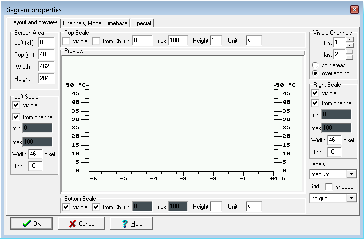
The Screen Area defines position (x1,y1) and size (width,height) of the diagram area. Changes in these fields immediately affects the preview.

The four scale controls on this tab define if and how axises are drawn at the left, right, top or bottom edge of the diagram area. The "size" parameter is either the width or height of the scale area, measured in pixels.
If a checkmark "from channel" is set, the value range for the scale labels is taken from the channel definition (on another tab). If it is not set, you can enter arbitrary values which do not necessarily match the value range of the parameter. This is frequently used to draw a "percentage" scale, for example if multiple channels with different scaling (or units) shall be displayed in the same diagram.
If the option "from channel" is not checked, you cannot enter arbitrary min/max values a scale because those parameters will be copied from the channel definition; and for the horizontal scale at the bottom of an Y(t) diagram, the default unit will be "s" (seconds).

Note:

Changing the style of the scale-indicator does not affect the displayed value range ("zoom factor") of the graph ! To change the displayed value range, use the "min"/"max" values on the tabsheet "Channels".

n

nano ( X * 10^-9 )

u

micro ( X * 10^-6 )

m

milli ( X * 10^-3 )

k

kilo ( X * 10^3 )

M

Mega ( X * 10^-6 )

G

Giga ( X * 10^-9 )

On tab 'Visible Channels' you select which of the 8 diagram channels shall be visible in the current diagram (there is a total of 8 channels; shared by all diagrams of your application as explained later). In X/Y-mode, the first channel will be the "X"-channel, the second the "Y"-channel. In Y(t)-mode, the first channel will be the upper curve if 'split areas' are selected. In 'overlapping areas' mode, all curves are plotted into a common diagram area - which can be confusing on a monochrome display sometimes. You should use different channel graph styles in this case as explained later.

Three different font sizes can be selected to add Labels to the scales of your diagram, or -alternatively- the numeric labels can be turned off (for all scales of the diagram) by selecting "no labels" in the "Labels" combo.
Note: If the 'size' of a scale is very small, the labels are automatically turned off for that particular scale. The drawing routine will not try to squeeze numeric labels into a too small scale area. This trick was used in the example shown above, where the sizes of the upper and right scale are only two pixels.

An optional grid can be turned on for the diagram's graph area. You can select no grid, vertical, horizontal, or both. The grid can be drawn either as solid lines or "shaded" (which is a fine-pitched dotted line for monochrome displays, which appears gray from some distance).

Channels, Mode, Timebase

On the second tab sheet, the data channels and some other diagram options can be defined:

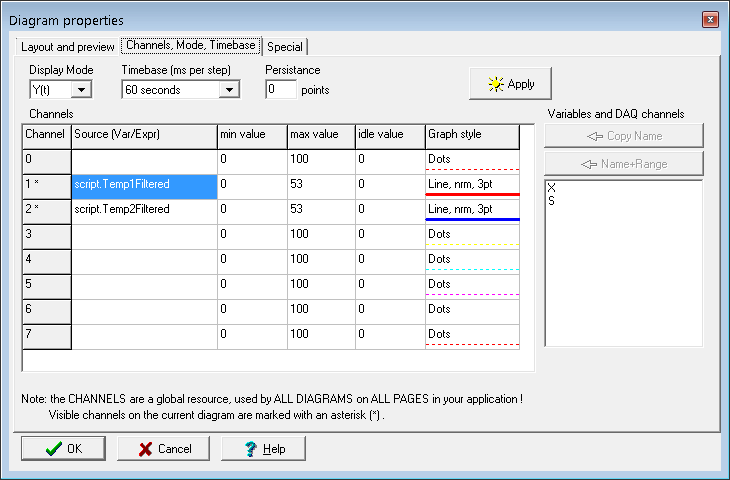
The controls on this tab sheet are:

Display mode

Can be set to Y(t) or X/Y. In X/Y-mode, the first channel of the diagram controls the X-axis, the second channel the Y-axis. In Y(t)-mode, the time dependent behaviour of all channels of the current diagram is displayed (X-axis = time).

Timebase

defines the update interval (usually a few ten milliseconds). In Y(t)-mode, a horizontal step of one graphic pixel is done per interval. In X/Y-mode, this interval - together with the "Persistance" value- defines how long old it takes until old points disappear from the screen (unless the special option "don't clear old curve" is selected).
If any of the diagram's channels is connected to the DAQ-unit, then the DAQ-unit's sampling rate may be automatically adapted to match the diagram's timebase.
Don't miss the notes about 'fast sampling' diagrams here !

Persistance

Only used for X/Y mode. Defines how many "old points" (or polygon segments) are visible on the screen. Must be between 1(*) and 255. If, for example, the Timebase parameter is set to 5*10 milliseconds, and "Persistance"=100, a new point will be drawn every 0.05sec, and will disappear from the diagram screen after 5 seconds (100 points * 0.05 seconds).
(*) Note: A persistance value of 1 (ONE) is only allowed if the graph style is set to "single dots". If the points of the graph shall be joined with lines, the persistance value must be 2 (TWO) or more.

Source (in the diagram-channel definition table)

Defines the origin of the samples in this channel. Usually, this will be the name of a display variable, but it's also possible to enter a short numeric expression in this column (which may call one of the interpreter's numeric functions).
By virtue of the DAQ unit, diagrams can also plot the waveform from an analog input (onboard), with a relatively high sampling rate (as far as the A/D converter + the DAQ permit).
Besides display variables and DAQ channels, diagrams can also directly show values from arrays declared in the script. References to such arrays are listed as script.<name>, where <name> is the name of a script variable declared as a one-dimensional array.
See also: Note about the 'early start' of data acquisition for diagrams since 2018-09-26,
                Note about plotting data from script arrays.

Min Value, Max Value (in the diagram-channel definition table)

Defines the graphic display range for a channel. You can use this to zoom into a certain range of interest. This range may affect the numeric labels on a vertical scale (if the checkmark "from channel" is set for a vertical axis).
When defining a new data channel, the min/max value are usually copied from the propierties of an UPT-variable, because a diagram input channel is usually connected to one of the UPT's user-defined variable. If you want to display more than one channel in the same diagram area, you should use a common value range. If this is not possible, use a simple common scale ("percentage") for the diagram and clear the checkmark "from channel" on the control panel for left+right scale.
For very special applications, you can also set (overwrite) these parameters with an interpreter command.

Graph Style (in the diagram-channel definition table)

Defines how the samples from this channel shall be drawn on screen (line style and thickness). In Y(t)-mode, this may be "single dots", "lines" (vectors, drawn-through or dotted), "black fill" or "gray filling pattern". To modify this, double-click into this cell (row+column) of the definition table. In X/Y-mode, only "dots" and "lines" are supported (but no filled areas). The line strength ('thickness') also applies to single dots. For example, this allows you to have a single, large dot moving around the screen (use persistance=1 for this).

Copy Name / Copy Name+Value Range

Copies the name of a variable (and optionally its value range) from the list of variable names into the currently selected channel definition line.

Notes:

• The "source" for a diagram data channel is usually a variable, but that is not necessarily the case. You can enter any numeric expression in the "Source" column, for example "sys.vsup" if you want to plot the terminal's own supply voltage, etc etc.
• The values shown in a diagram are internally stored in an array ('sample memory'). Data acquisition into these arrays starts as soon as a diagram gets visible. Data acquisition into these arrays begins shortly after power-on (the firmware scans all display pages for diagram channel definitions, which contain info about the "source" and the desired sampling rate). If the source is a normal variable, the array will be updated (in the background) even if the page with the diagram is not visible. As soon as the the page with the diagram gets visible, the diagram will be updated using the sampled values stored in the channel's internal array.
• Without the aid of the Data Acquisition Unit (DAQ), the maximum sampling rate is limited by the speed of the main loop. Depending on the complexity of the display, a main loop may take 100 milliseconds. Thus to achieve sampling rates of 10 Hz (and more) without drop-outs, use the DAQ as source (sample memory) as explained in chapter 2.4, for all channels that require 'fast sampling'.

Special diagram options

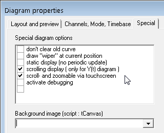
(Screenshot of the 'Diagram' dialog with the 'Special' tab opened)

Up to now, the following special options can be modified on the 3rd tab:

• don't clear old curve
  Can be used for unattended long-term observations. It may help you to see sporadic "runaways" (like unusual peaks in an otherwise flat line).
• draw "wiper" at current position ("windscreen wiper")
  Draws a thin vertical line at the current plotting position in Y(t)-mode. No effect in X/Y mode.
  Since 2016-08-04, the wiper's horizontal position is not reset when re-drawing a display page completely anymore. Instead, the position is only reset when switching from one display page to another, or when clearing the curve via command dia.clear.
  If the diagram is configured as 'scrolling', the windscreen wiper has no function, because new data always appear at the right edge of the diagram.

  Note about 'Windscreen Wiper' vs 'scrolling display':

  The non-scrolling 'windscreen wiper' is an anachronism for old 'passive STN' LCDs, and only still supported to remain compatible with old devices like 'MKT-View I'. The TFT displays in modern devices are fast enough even below the freezing point, thus for new applications, don't use the 'non-scrolling display with windscreen wiper' anymore. Use the scrolling display instead (details further below).

• static display (no periodic update)
  For 'very special' applications, in which the display shall not be updated (redrawn) 'automatically', but (for example) only via command in the script.
• scrolling display (only for Y(t) diagramm)
  With this option, the entire curve plotting area scrolls along the timescale (from right to left). The latest (newest) sample will always appear on the right edge of the plotting area.
  No effect in X/Y mode.
• scroll- and zoomable via touchscreen
  Allows the operator to modify the displayed value range at runtime. For details, see chapter 3.
• start acquisition only if this diagram gets VISIBLE
  Check this option if you need the old behaviour of a diagram, where data acquisition (for all channels connected to the diagram) did not start immediately after power-on.
  
• enable debugging
  Please don't. This option is only intended for software development.
• Background image (tCanvas)
  Optional image to fill the background of the diagram's curve area, generated by the script at runtime. Without a background image, the curve area will be filled with the background colour.
  In the following screenshot from application DAQ_Test.cvt, the diagram shows the microphone input in the time domain (red trace), the momentary spectrum (green trace), and the chronological sequence of audio spectra as a spectrogram (aka 'waterfall display') in the background of the curve area. For that purpose, the script uses a tCanvas for the spectrogram and the fast Fourier transform (FFT) to calculate the short-time spectra.
  

  
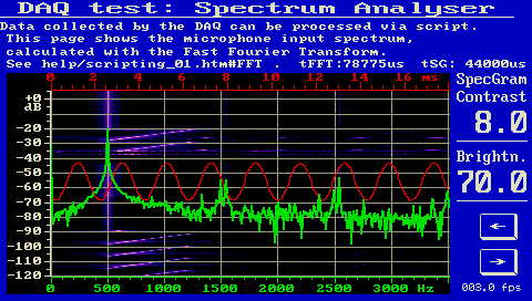
  Example for a diagram with background image (here: spectrogram from 'DAQ_Test.cvt')

back to top

Configuration of a 'fast sampling' diagram using the Data Acquisition Unit (DAQ)

Plotting values from script arrays

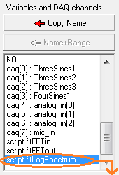
Selection list with data sources for a diagram,
including a few script variables (arrays)

const
   C_FFT_SIZE=1024; // number of samples for the FFT in the time domain, 2^N
endconst;

   ...

var
   float  fltFFTin[C_FFT_SIZE];       // FFT input (N real time domain samples)
   float  fltFFTout[C_FFT_SIZE+2];    // FFT output (N+1 complex frequency bins for the REAL FFT)
   float  fltLogSpectrum[C_FFT_SIZE/2]; // logarithmized amplitude spectrum (dB "over" full scale)
   float  re,im,mag,ref;
   int    i;
endvar;

    ...
  daq.read_channel( 7, fltFFTin );  // read input for the FFT from the DAQ into an array
  Math.rfft( fltFFTin, fltFFTout ); // Fourier Transform with real input, complex output
    ...
  display.UpdateDiagram; // update diagram AFTER the new set of data is complete
    ...

Retrieving diagram channel memories 'as text' (in the programming tool)

'empty':

This channel memory currently doesn't contain any sample,
for example because it's not being used by a diagram at all or its contents have been erased via command dia.clear.

'stopped':

This channel memory is currently not being filled with new samples,
for example because it's not being used by a diagram at all or it has been stopped via command (e.g. dia.run=0).

'running':

This channel memory is being fed with new samples, depending on its sample rate.

Zooming and panning (scrolling) a diagram via touchscreen

In devices with touchscreen, the operator may zoom into the diagram, or pan (scroll) the displayed value range as explained further below. To offer this feature, on the 'Diagram Properties' dialog, switch to the 'Special' tab, and set option
    scroll- and zoomable via touchscreen.

When enabled, the option allows to control Y(t)-diagrams as follows:

• Via touchscreen, vertical scales can be grabbed and moved up and down to shift the displayed display range of the ordinate ("Y axis").
  The diagram's curve are will be scrolled along with the scale(s).
  
• In Y(t)-diagrams with a visible horizontal time scale (i.e. physical unit set to "s" for "seconds"), the diagram can be shifted along the time axis by grabbing and moving the time scale via touchscreen. If data for the shifted range are available in the channel memories, the curves will scroll along with the timescale. Otherwise ('no data available' for a certain point in time), the curve remains empty, but will eventually be filled since the diagram's data acquisition keeps running in the background.
  As explained in chapter 2, a time scale with unit set to "s" in the designer doesn't mean the labels will always show 'seconds' - instead, the labels may show milliseconds, minutes, or even hours instead. But in any case, the value 'zero' represents the current date and time ("now") on this 'relative' timescale, and negative values represent the past.
  
• To zoom in and out, press the touch pen (or your finger) on the scale two times in a short time ^(*). On the second tap, hold it pressed. Then move the pen up to zoom in (expand), or down to zoom out the displayed range.
  The initially touched position remains in the center of the zoomed range.
  
• (with multi-touch capable hardware, you would be able to zoom into the diagram as you would on a smartphone or tablet PC, by two-finger-spreading gesture over the to-be-magnified object. But at the time of this writing (2018-08), only a single prototype with multi-touch display existed.)
• To switch back to the original ("designed") display ranges, rapidly ^(*) tap on the diagram's scale three times.

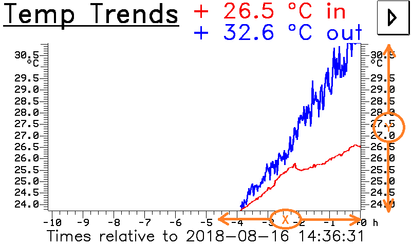
Scrollable Y(t) diagram from application script_demos/Thermo.cvt.
Orange circles and arrows mark the touchable areas for zooming,
or for scrolling along the horizontal (X) or vertical axis (Y).
Touchscreen events inside the curve area are reserved for the 'readout' feature (marker, cursor).

Sample memory (for zooming and scrolling diagrams)

Commands to control a diagram at runtime

dia.clear             (display interpreter command)
display.dia.clear      (script command)

This command erases the old graph in the diagram. In Y(t)-mode a new scan begins at the left side of the graph area. The grid (if enabled) will be redrawn immediately. All samples stored in channel memories (arrays) assigned to the diagram on the current display page are lost. Channel memories that are only used by disagrams on other display pages are not affected by this command.

dia.run=X             (display interpreter command)
display.dia.run := X    (script command)

This command stops and restarts the diagram display routine. "dia.run=0" means "Pause" (no more update of the visible diagram), "dia.run=1" or simply "dia.run" means "end of the pause, continue to update the diagram".
The current state (diagram stopped / running) can be queried with the function "dia.run". The following example shows how to toggle the "running" state:
dia.run=!dia.run
(the operator "!" means "boolean negation").

dia.ready             (display interpreter function)
display.dia.ready       (script function)

This function returns the diagram's scan-complete flag. It can be used to implement a single-shot diagram which can be started by the user and stops automatically when the scan reaches the end of the timebase. Use dia.ready in an event definition, and dia.run=0 as the reaction. This stops the diagram after a single scan. An example can be found in the file "diag_test1.cvt".
This flag is cleared automatically with the command dia.clear and dia.run.

display.dia.unix_time   (script function)

Returns the absolute timestamp (in "seconds elapsed since 1970-01-01 00:00:00") of the sample displayed on the left edge of the curve area). Unless the Y(t)-diagram was 'scrolled back in time', the result is almost identical to
  system.unix_time - display.dia.timespan_sec
Note: At the time of this writing, display.dia.unix_time was a read-only parameter. It cannot be used to horizontally scroll the diagram, but is affected by scrolling or zooming.

display.dia.timespan_sec   (script function)

For Y(t) diagrams, returns the "visible width of the curve area" in seconds.
This read-only parameter depends on the width of the diagram in pixels, but also from the timebase setting, and the magnification via touchscreen.

dia.plot_daq          (display interpreter command)
display.dia.plot_daq    (script command)

Plots the most recent data collected by the data acquisition unit (DAQ) into the diagram.
Side effect: The diagram is switched into a 'static' mode, without dynamic plotting.

dia.ch[N].min, dia.ch[N].max                (display interpreter read- and writeable parameters)
display.dia.ch[N].min, display.dia.ch[N].max   (script read- and writeable parameters)

Access to the channel scaling parameters during runtime. Can be used to "zoom" into the diagram area. Overwrites the channel's min/max parameters which were designed at design-time. The channel index (N) is the same as on the "Channels, Mode, Options" tab, the index begins at 0 (zero) for the first channel !
To zoom into an X/Y diagram, you must assign new values to four of these parameters ! Depending on which channel is connected to the X- and which to the Y-axis, these may be dia.ch[0].min, dia.ch[0].max,  dia.ch[1].max, and dia.ch[1].max . The diagram will be automatically redrawn if you assign new values to the channel's scaling parameters.
To revert to the channel scaling parameters at design time, use the command dia.ch[N].reset .
When zooming or scrolling the diagram via touchscreen, these values may change at runtime.

dia.ch[N].reset                          (display interpreter command)
display.dia.ch[N].reset                    (script command)

Reverts to the channel scaling parameters at design-time. Can be used to "zoom out" after modifying the diagram's scaling parameters with the commands dia.ch[N].min and dia.ch[N].max .

dia.ch[N].n_samples                       (read only)

Returns the number of samples currently stored in channel 'N'. Only for diagnostic purposes, for example to examine channels in the Watch-window.

dia.sc.X.min,  dia.sc.X.max                 (display interpreter read- and writeable parameters)
display.dia.sc.X.min,  display.dia.sc.X.max    (script read- and writeable parameters)

Modifies one of the numeric scales of a diagram during runtime, but not the transformation parameters for a data channel. X: l=left, r=right, t=top, b=bottom . Only works if the scale is not associated to a channel (which means, the checkmark "from channel" must not be set for this scale) ! Example:
dia.sc.t.min = -1.5 : dia.sc.t.max = 100.0

Polygons in the curve area of a diagram

dia.poly(from_row, to_row, from_column, to_column)         (display interpreter command)
dia.poly(arr[from_row~to_row][from_column~to_column])   (display interpreter command)
display.dia.poly[N].draw( <source_array>, <options> )   (script command)

Draws a closed polygon in the plotting area of the diagram. The polygon coordinates are usually copied from an array (for the display interpreter, there's only a global array). The second notation (with the explicit specification of the array's name) is the preferred syntax (and in the script, the only possible form). Example for the display interpreter:
dia.poly(arr[0~8][0~3])
Draws nine polygons, using rows 0..8 in the global array; with four points each, stored in in columns 0..3 of the array.
Note: The array must be filled with the point coordinates before this command is invoked ! How to fill the array is explained in a separate document for the display interpreter, and here for the script language.
For individual control, you can specify which of the diagram's polygons(*) shall be drawn, and for clarity, you can add the token ".draw" after the polygon index. Example for the display interpreter:
dia.poly[9].draw(arr[10][0~3],o) draws polygon #9 only, using the 11-th line of the array, as an OPEN polygon (lower case 'o' at the end)

^(*) The number of polygons per diagram is limited to 20, even though the capacity of the array which holds the polgon coordinates may be larger. Thus, the maximum polygon index -also for the commands further below- is 19 because array indices begin at zero.

dia.poly.clear                     (display interpreter command)

Removes all polygons from the diagram's plotting area.

dia.poly[N].dmode=<draw mode>         (display interpreter command)
dia.poly.dmode                     (display interpreter function)

Changes the display mode for the polgon on a monochrome display. N is the polygon index (counting starts at zero, N=0 is the FIRST polygon, max index is specified here). Usable draw modes are: 0=solid, not blinking, 1=blinking in page 1, etc). The polygon index can be left out to change the appearance of all polygons with a single command.
For colour displays, the 'draw mode' has no effect. Use different colours instead.

dia.poly[N].color=<color>             (display interpreter command)

Changes the the colour of the specified polygon's lines (if the device has a colour display).  If no particular polygon index (N) is specified, the command sets the colour for all polygons currently visible. An overview of all usable colours can be found here .

dia.poly[N].width=<line width in pixels>   (display interpreter command)
dia.poly.width

Changes the width ("thickness") of the polygon lines in pixel. The polygon index can be left out to change the appearance of all polygons with a single command. Use this feature economically, because too wide lines may slow down the screen update rate. The default line width is 1 (one) pixel.

dia.poly[N].text="<string>"           (display interpreter command)

Prints a short text message (max. 8 characters) close to the specified polygon. The text must be specified with this command before the polygon is drawn into the diagram. Defining the string during runtime is not possible. Note that the number of polygons per diagram is limited.

Other commands to control the diagram may follow in future.
An example for advanced users with runtime-generated polygons in a diagram can be found in the application MKTview2/MV2_Poly.cvt.

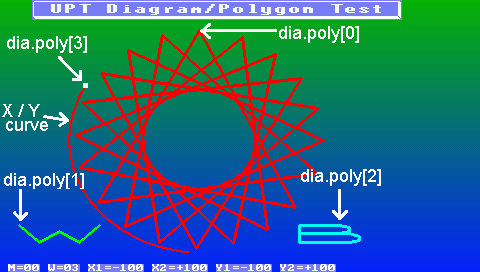
Screenshot from application 'programs/MKTview2/MV2_Poly.cvt'
(Test for diagrams with polygons in the curve area, here on an MKT-View III)

  Event     Reaction
  always    arr[4][0][0~1]={X,Y};         // copy X and Y into the array (one point)
  always    dia.poly[3].color = white : dia.poly[3].width = 5; // prepare drawing ..
  always    dia.poly[3].draw(arr[4][0][0~1],o); // draw X,Y as polygon with a single point 

Drawing polygons in diagrams via script

 display.dia.poly[Index].draw( <Source> [,Colour][,Text][,Options] )
                    |             |         |      |      |
                    |             |         |      |      |__ optionale flags
             polygon index,       |         |      |
             optional, 0..19      |         |      |__ optional text string, to be
                                  |         |          displayed 'near the polygon'
                                  |         |__ optional specification of a colour
                                  e.g. an array, optionally with the number of points

var
   float PeakIndicator[3][5][2];
         //            |  |  |___ coordinate : 0=x, 1=y (least significant dimension)
         //            |  |______ point index (here, up to 5 points per polygon)
         //            |_________ polygon index : 0..2 (for up to 3 polygons)
endvar;

  display.dia.poly[0].draw( PeakIndicator[0], 3, clRed, "Indicator 1", pfClosed ); 
 //                         | source, here with|   |         |           |
 //                         |  number of points|   Colour    Text        |
 //                         |_______(optional)_|  (optional) (optional)  |
 //  ____________________________________________________________________|
 // |
 // |
 // Option (optional:o)

See also:

Polygons outside a diagram, created with the graphic editor
back to top

Diagram-specific event handling in the application's script

func OnDiagramTouchEvent( int event, int area, float scaled_x, float scaled_y ) // touch event in a diagram

This handler will be invoked by any kind of touchscreen-event within the diagram's client area. The first function argument informs the handler about the type of the event:

event : This integer value may be one of the following built-in constants:

evPenDown : "touchsceen was just pressed, with a coordinate within the diagram's area on the screen"
evPenMove : "pen or finger was moved, coordinate still within the diagram"
evPenUp   : "pen or finger was lifted from the touchscreen" (with the last valid coordinate inside the diagram)

curve_area : indicates the screen area within the diagram:

arLeftScale  : Vertical scale on the diagram's left side (for the 1st 'Y-axis')
arRightScale : Vertical scale on the diagram's right side (for the 2nd 'Y-axis')
arTopScale   : Horizontal scale at the top of the diagram
arBottomScale: Horizontal Scale at the bottom of the diagram ('X'- or time axis)
arCurve1 : first curve area (always present)
arCurve2 : second curve area (optional, for 'split' multi-channel diagrams)

scaled_x : horizontal position, same unit as the 'physical value(s)'.

In X/Y-diagrams, scaled like the values measured on the 'X'-channel.
In Y(t)-diagrams, 'x' is a time in seconds, same unit as in system.timestamp_sec and display.dia.timestamp_sec.

scaled_y : vertical position, same 'physical values' as measured values.

In X/Y-diagrams, matching the physical values measured on the 'Y'-channel.
In Y(t)-diagrams, same scaling as for 'physical values' in the first visible channel in the curve area.

Similar as in low-level event handlers like 'OnPenDown', 'OnPenMove' and 'OnPenUp', the return value from OnDiagramTouchEvent defines if the event has completely been handled completely in the script (return TRUE), or if the system's default-handler shall process it instead (return FALSE). If touchscreen events have already been 'intercepted' in one of the low-level event handlers listed above (via 'return TRUE' at the end of the event handler), then OnDiagramTouchEvent will not be called at all.

A simple example using 'OnDiagramTouchEvent' can be found in application script_demos/diagrams.cvt .

(*) In addition to the diagram-specific event handlers presented in this chapter, your script could also process touchscreen events in the unspecific OnControlEvent handler. But in that case, you would have to transform pixel coordinates into physical values "yourself", which is possible but tedious.

Syntax for a diagram in a backslash sequence

Internally, the diagram is coded as a backslash sequence. The UPT's interpreter analyses it just like any other format string in a display command. If you prefer writing the source code for a display page with a text editor instead of clicking it together, this is for you:

Syntax:

\dia( width,height, 1st_chn,last_chn,style,diagram_flags,timebase) (deprecated)
\dia2( 1st_channel,last_channel,style,diagram_flags,timebase)

This is the main diagram definition. For newer devices, width and height are not part of the argument list (in parentheses) anymore. Instead, they belong to the 'general properties' of any display element, which can be modified on the display line properties panel.

\dia.sc.X(scale_flags,size,min,max)

Definition of a diagram scale. 'X' may be 'l','r','t','b' (left, right, top, bottom) Parameters:
  scale_flags : Decimal parameter with bitwise endcoded flags for a certain scale.
    Bit 0 (mask 1) : 1=visible, 0=invisible
    Bit 1 (mask 2) : 2=min/max from a channel definition, 0=independent min/max-values.

  size :
    Width of a vertical, or height of a horizontal scale in pixels.
    0 = "automatic" (depends on the space required for ticks + labels + physical unit).

  min :
    Value for the label "at the lower end" (no effect if value range taken from a channel)

  max :
    Value for the label "at the upper end" (no effect if value range taken from a channel)

Optionally, a physical unit can be speficied as key=value pair (u="unit") after parameter 'scale_flags'. The unit (string) will be appended after the numeric label.

\dia.chX(graph_style,channel_flags,sampling_interval,min,max,idle)

Definition of a diagram data channel. 'X' may be '0'...'7' (channel index).
Parameters:
  graph_style : Decimal encoded parameter with multiple bitgroups:
    Bits 3..0 : Dot- or line pattern:
      0 = single dots,
      1 = continuous line,
      2 = filled area (only for Y(t)-diagrams, not for X/Y),
      3 = gray hatched area (for Y(t)-diagrams on monochrome displays),
      4 = dotted line,
      5 = slashed line.
    Bits 7..4 : Width of the line ("curve") in pixels.

  channel_flags :
    Old parameter, only exists for compatibility reasons.

  sampling_interval :
    Time step (interval) when "collecting" data for this diagram channel.
    This parameter may be specified in milliseconds ("ms"), seconds ("s"), or minutes (suffix "min").
    Without a suffix (unit), the sampling interval is interpreted as a multiple
    of 10 millisecond units (for compatibility with ancient "UPT" and "MKT-View" devices).

  min :
    Minimum value for scaling (lower edge of in the curve area).

  max :
    Maximum value for scaling (upper edge of in the curve area).

  idle :
    This value will be entered in the diagram's sample array,
    if no valid data are available (e.g. missing data from CAN).

Most of the arguments (parameters) are the same properties as mentioned earlier. These definition lines are generated automatically when the user clicks "OK" in the diagram definition dialog shown in chapter 2. Older definition lines (in the display-definition table) are overwritten in that case.

The scale ranges (scale_min and scale_max) may only be defined in the backslash sequence if the min/max-values are NOT taken from the variable definition.

If you need further information, please get in contact with the author of this software.

Last modified: 2018-12-08 by WB / MKT Systemtechnik .

• Diagrams: Overview
• Configuration
• Layout and Preview
• Channels, Mode
• Options
• Polygons
•